How to model dwell time of proteins on DNA binding sites in R - part 1

July 19, 2014

Disclaimer: In this post i’m working through my own thinking on how to think about and model simple dwell times of proteins on their DNA binding sites. I’m not sure any of this is correct (yet).

Statistical interpretation of protein dissociation

Let’s consider an individual protein bound to DNA that is observed at fixed time intervals of \(t_i = 0.1s\) by single molecule imaging. At each of these steps there is a certain probability \(p_d\) that the molecule dissociates from the DNA. This can be modelled as a bernulli process that is repeated until one decay event (i.e. dissociation) has been observed, which means that the number of time steps until dissociation should follow a negative binomial distribution with a “success rate” (i.e. probability of staying bound) of \(p_{nd} = 1 - p_d\).

The mean of the negative binomial distribution is

\[\mu = \frac{p_{nd}}{1-p_{nd}}\].

Therefore, if a protein has a mean dwell time of 10s at a given site, the probability of dissociation during any time step \(t_i\) would be

\[\begin{aligned} \frac{p_{nd}}{1-p_{nd}} &= \frac{10}{0.1} \\ p_{nd} &= \frac{100}{101} \\ p_d &= 1 - \frac{100}{101} \approx 0.0099 \\ \end{aligned} \]

Similarly, for a mean dwell time of 1s, \(p_d \approx 0.09091\).

Simulating a single high affinity site model

Based on the previous section, dwell time data can now be modeled for a single high affinity site with a mean dwell time of 10s and a total of 2000 bound sites (without actually using the neg. binomial distribution). A term for measurement error is introduced as well.

set.seed(13219)
dt.1 <- c()
ti <- 1
n  <- 2000
pd.ha <- 1 - 100/101
while (n > 0) {
  n.diss <- min(sum(runif(n) <= pd.ha), n)
  n <- n - n.diss
  dt.1 <- c(dt.1, rep(ti, n.diss) + round(rnorm(n.diss, sd=2)))
  ti <- ti + 1
}
dt.1[dt.1 < 1] <- 1

Plotting the distribution of dwell times

library(ggplot2)
p <- ggplot(data.frame(dt=dt.1)) +
  geom_histogram(aes(x=dt), fill="grey70", color="black", binwidth=5) +
  labs(x=expression(paste("Dwell time x", 10^{-1}, "s")), y="n") + 
  theme_bw(16)

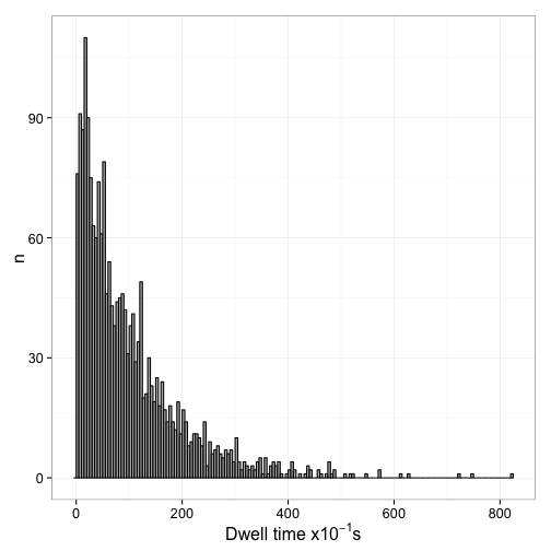
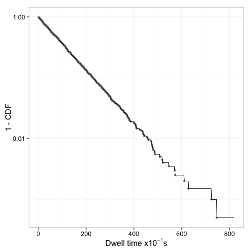
plot of chunk 2014-07-22-fig1 — **Figure 1**: Distribution of dwell times

Now we can interpet this from the view of the whole population of sites. Essentially, unlike what happens in the single molecule tracking, we assume that we started with all sites bound and then observe the decrease of bound sites over time. This is equivalent to shifting all dwell times overved at different times in the experiment to a start time of 0. The easiest way to do this is essentially calculating an empirical CDF function of the dwell times:

dt.1.cdf <- ecdf(dt.1)

Next, we create a data.frame that gives unique values of dt.1 along with 1 - CDF (unique values only since there are many ties in the data).

dt.1.u <- unique(dt.1)
dt.1.df <- data.frame(t = dt.1.u,
                      mcdf = 1 - dt.1.cdf(dt.1.u))
dt.1.df <- subset(dt.1.df, mcdf > 0)

Figure 2 shows that 1 - CDF indeed appears to be an exponential decay.

plot of chunk 2014-07-22-fig2 — **Figure 2**: 1 - CDF. Shown in grey dots is the estimate at the original data locations. Shown as a line is evenly spaced data every two time steps. Note that `ecdf` creates a stepfunction.

Fitting a single exponential model

Linearize data and fit by linear regression

The exponential decay function

\[n(t) = n_0\cdot e^{-\frac{t}{\tau}}\]

where \(\tau\) is the mean dwell time can be linearized

\[\begin{aligned} log(n(t)) &= log(n_0\cdot e^{-\frac{t}{\tau}}) \\ &= log(n_0) - \frac{1}{\tau} \cdot t \\ &= log(n_0) - \lambda \cdot t \\ \end{aligned} \]

and the linearized model can be fit to transformed data:

dt.1.df$log.mcdf <- log(dt.1.df$mcdf)
linm <- lm(log.mcdf ~ t, data = dt.1.df)
summary(linm)

## Call:
## lm(formula = log.mcdf ~ t, data = dt.1.df)
## 
## Residuals:
##     Min      1Q  Median      3Q     Max 
## -0.2550 -0.0104  0.0014  0.0143  0.4350 
## 
## Coefficients:
##              Estimate Std. Error t value Pr(>|t|)    
## (Intercept)  3.96e-03   3.95e-03       1     0.32    
## t           -1.01e-02   1.63e-05    -623   <2e-16 ***
## ---
## Signif. codes:  0 '***' 0.001 '**' 0.01 '*' 0.05 '.' 0.1 ' ' 1
## 
## Residual standard error: 0.0425 on 353 degrees of freedom
## Multiple R-squared:  0.999,	Adjusted R-squared:  0.999 
## F-statistic: 3.88e+05 on 1 and 353 DF,  p-value: <2e-16

results in the expected mean dwell time of \(\tau = \frac{1}{\lambda} =\) 98.5474 and an intercept of 1.004.

However, the diagnostic plots for the linear regression on transformed data suggest that some assumptions are being violated (see Figure 3).

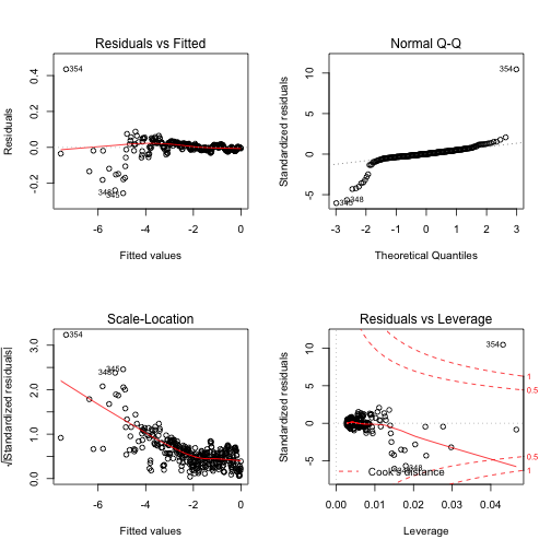
plot of chunk 2014-07-22-fig3 — **Figure 3**: Diagnostic plots for the linear regression on transformed data

There are several issues i can think off that may play into this:

because of the nature of the data generating process, there are many more data points to the left of \(\overline{X}\) than there are to the right
the linearization has to assume that the error is multiplicative, but the data generation process has an additive error term
the data is discrete
the noise in the data is unrealistically low.

The second and third term cannot be easily fixed. However, what would happen if the 1 - CDF data was replaced by a fixed, evenly spaced number of linearly interpolated data points?

eq.spaced <- seq(min(dt.1), max(dt.1), by=1)
df.eq <- data.frame(t=eq.spaced, mcdf=approx(dt.1.u, 1 - dt.1.cdf(dt.1.u), 
                                             xout=eq.spaced)$y)
df.eq <- subset(df.eq, mcdf > 0)
df.eq$log.mcdf <- log(df.eq$mcdf)
linm.i <- lm(log.mcdf ~ t, data = df.eq)
summary(linm.i)

## Call:
## lm(formula = log.mcdf ~ t, data = df.eq)
## 
## Residuals:
##    Min     1Q Median     3Q    Max 
## -3.423 -0.048  0.007  0.073  0.581 
## 
## Coefficients:
##              Estimate Std. Error t value Pr(>|t|)    
## (Intercept)  8.19e-02   2.06e-02    3.98  7.5e-05 ***
## t           -1.05e-02   4.35e-05 -240.58  < 2e-16 ***
## ---
## Signif. codes:  0 '***' 0.001 '**' 0.01 '*' 0.05 '.' 0.1 ' ' 1
## 
## Residual standard error: 0.294 on 817 degrees of freedom
## Multiple R-squared:  0.986,	Adjusted R-squared:  0.986 
## F-statistic: 5.79e+04 on 1 and 817 DF,  p-value: <2e-16

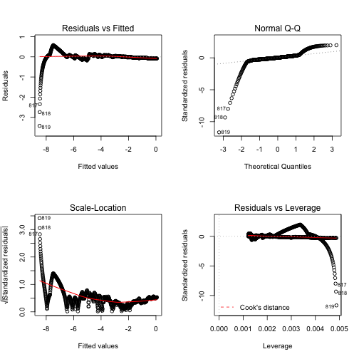
Figure 4 shows the diagnostic figures for this fit. This certainly didn’t help any.

plot of chunk 2014-07-22-fig4 — **Figure 4**: Diagnostic graphs for linear fit to transformed, equally spaced data (linear extrapolation)

Directly fit exponential model

In our specific case, since we are studying a CDF, \(n_0 = 1\), which means that the exponential that we are fitting is

\[n(t) = e^{- \lambda t}\]

We fit this to the original data using the base R nls function

expm <- nls(mcdf ~ exp(- l*t), data=dt.1.df, start=list(l=1/5))
summary(expm)

## Formula: mcdf ~ exp(-l * t)
## 
## Parameters:
##   Estimate Std. Error t value Pr(>|t|)    
## l 1.01e-02   7.76e-06    1308   <2e-16 ***
## ---
## Signif. codes:  0 '***' 0.001 '**' 0.01 '*' 0.05 '.' 0.1 ' ' 1
## 
## Residual standard error: 0.00366 on 354 degrees of freedom
## 
## Number of iterations to convergence: 6 
## Achieved convergence tolerance: 2.7e-06

Again, the estimate for the mean dwell time of 98.6092 is close to the real value of 100.

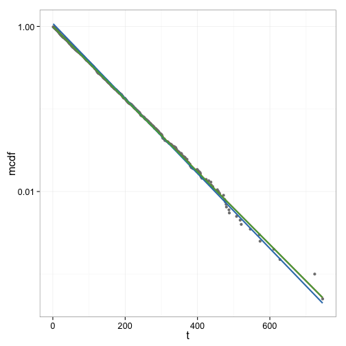
Figure 5 shows the curve fits done so far in one graph for comparison. In this data set as well as several others the difference between the linear fit and the exponential fit is small. The fit to the linearly interpolated CDF data however appears to be less good.

plot of chunk 2014-07-22-fig5 — **Figure 5**: Original data: **grey dots**; linear fit on transformed original data: **red line**; linear fit on transformed original data, equally spaced by interpolation: **blue line**; direct exponential fit: **green line**. The green and red line are not distinguishable.

Simulating a mixture of high and low affinity sites

Next, data for a mixture of a high affinity site (mean dwell time of 10s, 200 sites) with low affinity sites (mean dwell time of 1s, 1800 sites) is simulated using a similar process as above

set.seed(5620)
sim.2.data <- function() {
  dt.2 <- c()
  ti <- 1
  n.la  <- 1800
  n.ha  <- 200
  pd.ha <- 1 - 100/101
  pd.la <- 1 - 10/11
  while (n.la + n.ha > 0) {
    n.diss.la <- min(sum(runif(n.la) <= pd.la), n.la)
    n.la <- n.la - n.diss.la
    n.diss.ha <- min(sum(runif(n.ha) <= pd.ha), n.ha)
    n.ha <- n.ha - n.diss.ha
    dt.2 <- c(dt.2, rep(ti, n.diss.la + n.diss.ha) + 
                round(rnorm(n.diss.la + n.diss.ha, sd=1.5)))
    ti <- ti + 1
  }
  dt.2[dt.2 < 1] <- 1
  dt.2
}
dt.2 <- sim.2.data()
dt.2.cdf <- ecdf(dt.2)
dt.2.df <- data.frame(t = unique(dt.2))
dt.2.df$mcdf <- 1 - dt.2.cdf(dt.2.df$t)
dt.2.df <- subset(dt.2.df, mcdf > 0)

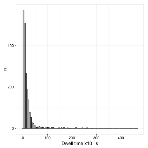
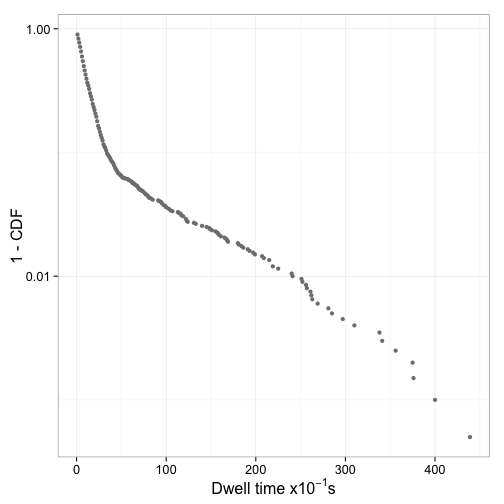
Figure 6 shows the distribution of dwell times and Figure 7 the log plot of 1-CDF of the dwell times

plot of chunk 2014-07-22-fig6 — **Figure 6**: Distribution of dwell times for mixed site model: 200 high affinity sites with a mean dwell time of 10s, 1800 low affinity sites with a mean dwell time of 1s.

plot of chunk 2014-07-22-fig7 — **Figure 7**: 1 - CDF of mixed model.

Fit mixed exponential model

The mixed exponential model that should be fit here is

\[n(t) = f_{ha}e^{-\lambda_{ha}t} + (1 - f_{ha})e^{-\lambda_{la}t}\]

This cannot be easily linearized. Therefore the exponential model needs to be fit directly. Again we use nls. However, keep in mind that there is no distinction between the two rate constants, which means that either one of them might end up corresponding to the high affinity sites.

expm.2 <- nls(mcdf ~ f * exp(- l1 * t) + (1 - f) * exp(-l2 * t), 
              data  = dt.2.df, 
              start = list(l1=1/10, l2=1/2, f=0.5))
summary(expm.2)

## Formula: mcdf ~ f * exp(-l1 * t) + (1 - f) * exp(-l2 * t)
## 
## Parameters:
##    Estimate Std. Error t value Pr(>|t|)    
## l1 0.009268   0.000234    39.6   <2e-16 ***
## l2 0.095546   0.000385   248.0   <2e-16 ***
## f  0.092851   0.001809    51.3   <2e-16 ***
## ---
## Signif. codes:  0 '***' 0.001 '**' 0.01 '*' 0.05 '.' 0.1 ' ' 1
## 
## Residual standard error: 0.00334 on 143 degrees of freedom
## 
## Number of iterations to convergence: 9 
## Achieved convergence tolerance: 5.46e-07

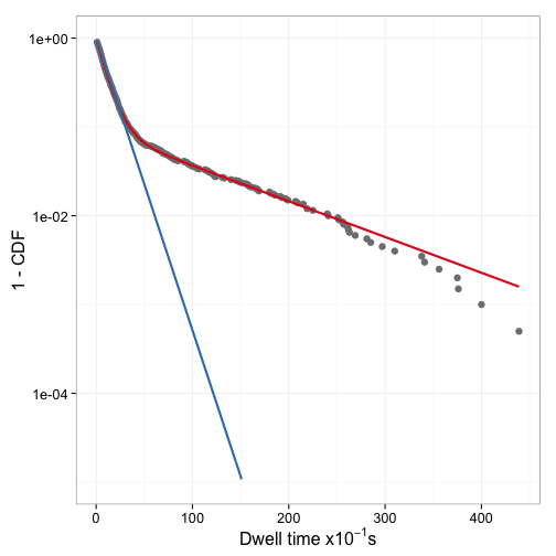
The estimates of the mean dwell time of the high affinity sites (107.903), the low affinity site (10.4662), and the fraction of sites that are high affinity (0.0929) are close to the values used in the data generating process.

Is the two component model significantly better than a single component model?

expm.2.single <- nls(mcdf ~ exp(-l * t), 
                     data  = dt.2.df,
                     start = list(l=1/10))
summary(expm.2.single)

## Formula: mcdf ~ exp(-l * t)
## 
## Parameters:
##   Estimate Std. Error t value Pr(>|t|)    
## l  0.07572    0.00125    60.3   <2e-16 ***
## ---
## Signif. codes:  0 '***' 0.001 '**' 0.01 '*' 0.05 '.' 0.1 ' ' 1
## 
## Residual standard error: 0.0301 on 145 degrees of freedom
## 
## Number of iterations to convergence: 6 
## Achieved convergence tolerance: 3.8e-06

anova(expm.2.single, expm.2)

## Analysis of Variance Table
## 
## Model 1: mcdf ~ exp(-l * t)
## Model 2: mcdf ~ f * exp(-l1 * t) + (1 - f) * exp(-l2 * t)
##   Res.Df Res.Sum Sq Df Sum Sq F value Pr(>F)    
## 1    145     0.1310                             
## 2    143     0.0016  2  0.129    5799 <2e-16 ***
## ---
## Signif. codes:  0 '***' 0.001 '**' 0.01 '*' 0.05 '.' 0.1 ' ' 1

Indeed it is. Figure 8 shows the two fitted models with the data.

plot of chunk 2014-07-22-fig8 — **Figure 8**: Mixture model with `nls` fit of 2 component model (red) and singe component model (blue). Since the low affinity sites are in excess, the single component model ends up being a reasonable estimate of the low affinity dwell time.

How dependent on the starting values are the results of nls? To find out, nls is run with a range of starting values for lla and lha (fixing f at 0.5).

fit.grid <- local({
  eg <- expand.grid(start.l1=10^seq(-3, 0, length.out=100),
                    start.l2=10^seq(-3, 0, length.out=100))
  eg$fit.l1 <- NA
  eg$fit.l2 <- NA
  eg$fit.f   <- NA
  for (i in 1:nrow(eg)) {
    fit <- try(nls(mcdf ~ f * exp(- l1 * t) + (1 - f) * exp(-l2 * t), 
               data  = dt.2.df, 
               start = list(l1=eg[i, "start.l1"], 
                            l2=eg[i, "start.l2"], 
                            f=0.5)),
               silent=TRUE)
    if (inherits(fit, "nls")) {
      eg$fit.l1[i] <- coef(fit)["l1"]
      eg$fit.l2[i] <- coef(fit)["l2"]
      eg$fit.f[i]   <- coef(fit)["f"]
    }
  }
  eg$fit.lha <- pmin(eg$fit.l1, eg$fit.l2)
  eg$fit.lla <- pmax(eg$fit.l1, eg$fit.l2)
  eg$fit.fha <- ifelse(eg$fit.l1 < eg$fit.l2, eg$fit.f, 1-eg$fit.f)
  eg
})

Figure 9 shows how the inital estimates for the parameters impact which of the two rate constants ends up estimating the high affinity sites and how many times the model fitting fails. Clearly the direction of the estimates and any estimates are possible at all heavily depend on the starting parameter estimates.

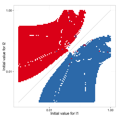
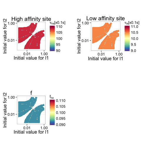
plot of chunk 2014-07-22-fig9 — **Figure 9**: Whether l1 is the estimate for the high affinity binding site (red) or not (blue) depends on the selection of the initial estimates in a mostly predictable way. Note that there are many combinations of initial estimates that yield no results due to a failure of `nls` (white).

Figure 10 shows how accurate the fitted values for high affinity mean dwell time, low affinity mean dwell time, and fraction of high affinity sites are as a function of the initial estimates. It is clear that in this particular data set, the bias of the estimates is not dependent on the initial input data.

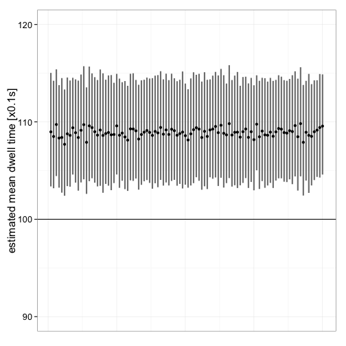
plot of chunk 2014-07-22-fig10 — **Figure 10**: Deviations of the estimates for mean dwell time of the high affinity site (top left), mean dwell time of the low affinity site (top right), and the frequency of high affinity sites (bottom left). In all cases, color scale is centered at the real value used in data generation. Red values indicate overestimates; blue colors underestimates. In the case of mean dwell time, an overestimate of the dwell time means that the rate constant was underestimated.

Another question is how good the estimates are for different data sets. So, 100 data sets are simulated and the estimates along with their confidence intervals are plotted. Initial values are selected based on the previous analyses. Figure 11 shows that the mean dwell time is consistently overestimated (rate constant underestimated), irrespective of data set. Despite the obvious bias, the difference is reatively small.

set.seed(3321999)
fit.rep <- list()
for (i in 1:100) {
  tmp <- sim.2.data()
  tmp.cdf <- ecdf(dt.2)
  tmp.df <- data.frame(t = unique(tmp))
  tmp.df$mcdf <- 1 - tmp.cdf(tmp.df$t)
  tmp.df <- subset(tmp.df, mcdf > 0)
  fit <- try(nls(mcdf ~ f * exp(- lha * t) + (1 - f) * exp(-lla * t), 
             data  = tmp.df, 
             start = list(lha=1/30, lla=1/3, f=0.5)),
             silent=TRUE)
  if (inherits(fit, "nls")) {
    fit.rep[[i]] <- fit
  }
}

plot of chunk 2014-07-22-fig11 — **Figure 11**: Point estimate and confidence interval of the dwell time for the high affinity site in 100 simulated data sets.

Final thoughts

There appears to be a consistant bias in the estimates. In a future post i will try to determine where the bias comes from (or if there is a flaw in the simulated data).
nls defaults to the Gauss-Newton algorithm which is less stable with respect to initial estimates than Levenberg-Marquardt (LM). minpack.lm provides the LM algorithm. In a future post i will compare nls to the minpack implementation as well s the gnm package, which implements generalized nonlinear models.